Understanding Stable Diffusion

In this blog post I will be presenting a high level explanation of what Stable Diffusion is and how it works. This is the insights I’ve got from Lesson 9 of the fast.ai 2022 part 2 course.

According to Wikipedia Stable Diffusion is a deep learning, text-to-image model released in 2022. It is primarily used to generate detailed images conditioned on text descriptions, though it can also be applied to other tasks such as inpainting, outpainting, and generating image-to-image translations guided by a text prompt. It was developed by researchers from the CompVis Group at Ludwig Maximilian University of Munich and Runway with a compute donation by Stability AI and training data from non-profit organizations.

The basic idea behind Stable Diffusion:

Basically what Stable Diffusion does is that it starts from random noise and each step tries to make it slightly less noisy and slightly more like the thing we want

You may be wondering now: - How can we go from that random noise to the actual image we want?

The way stable diffusion is usually explained is focused very much on a particular mathematical derivation. But in fastai developed a new way of thinking about Stable Diffusion, it’s mathematically equivalent to the classic approach, but is conceptually much simpler.

The Magic Function:

Let’s imagine that we are trying to get something to generate handwritten digits (stable diffusion for handwritten digits). How do we go about it?

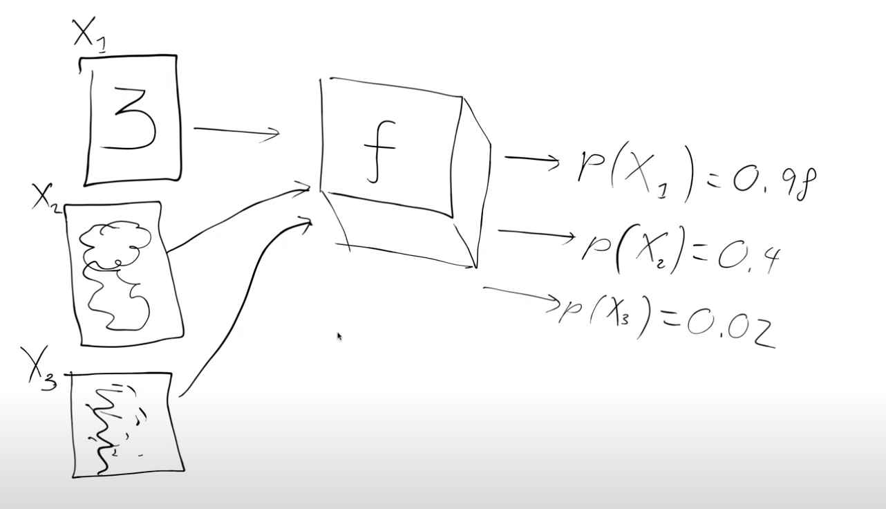
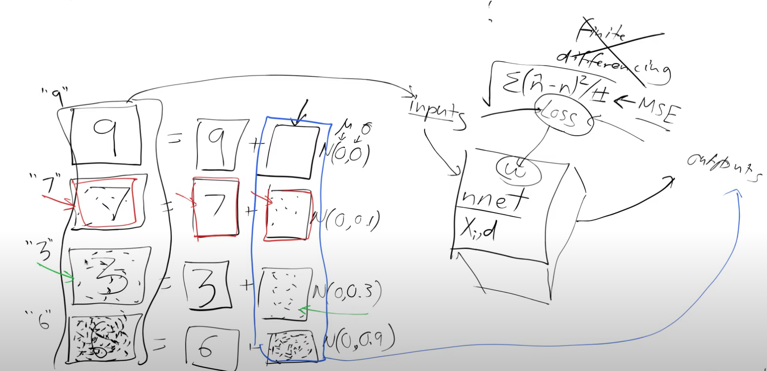
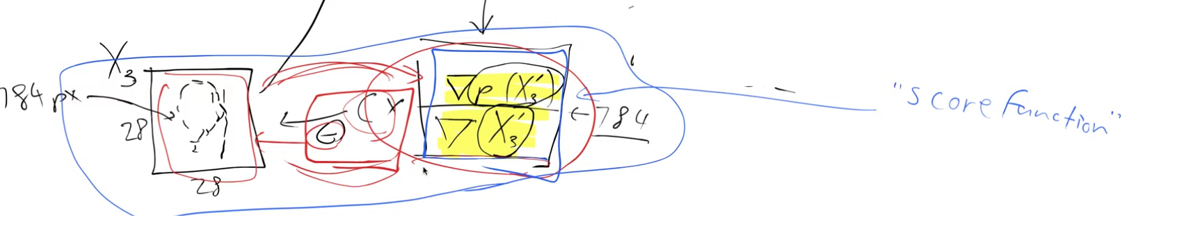
We’re going to start by assuming there’s some magic function \(f\) (black box for now), that takes in a handwritten digit and spits out the probability of it being a handwritten digit. For example we pass in an image \(X_1\) and it spits back p(\(X_1\)) = 0.88 i.e the probability that \(X_1\) is a handwritten digit, \(X_1\) corresponds to the digit 3 in the figure below

Why is this magic function interesting ? We can use it to actually generate handwritten digits.

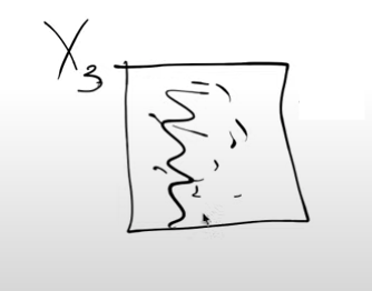
Image \(X_3\) in the figure doesn’t look like a digit. Let’s see how we could try to convert it into a handwritten digit. It is a 28x28 image with 784 pixels.

The idea is to slightly alter each of the pixels, and each time we alter a pixel we pass it to the magic function and see how the probability changes. We want to make changes to the image with the hope that the probability value of it being a handwritten digit increases.

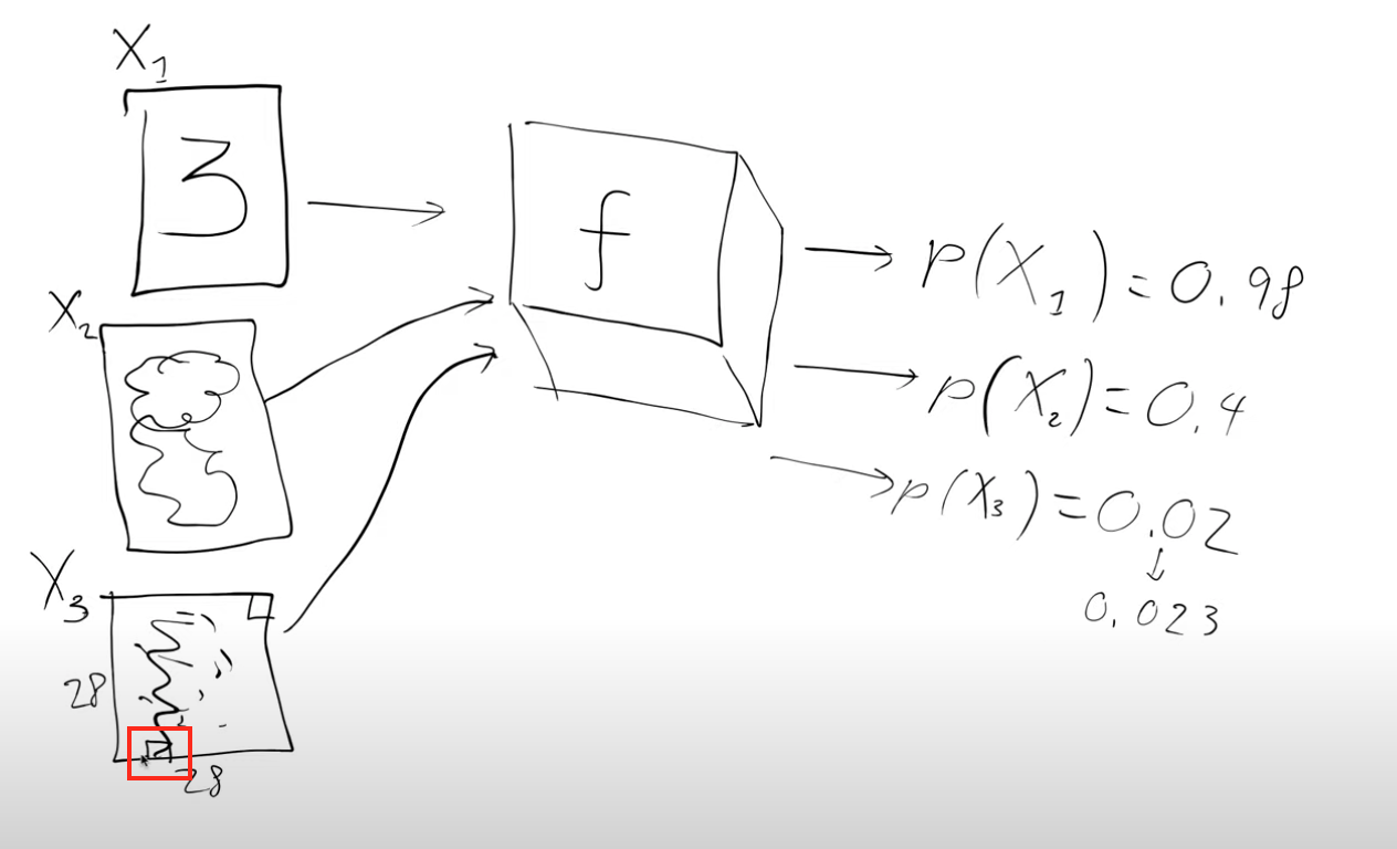
Let’s examine a specific instance, image \(X_3\), as an example. Normally, handwritten digits do not have any black pixels at the very bottom edge (marked by the red box). Hence, if we slightly brighten the image and run it through our magical function, the probability of it being recognized as a handwritten digit would likely increase marginally (for instance, from 0.02 to 0.023).

We can repeat this process for every individual pixel in the 28x28 image. The objective is to determine which pixels should be made slightly lighter and which ones should be darkened to enhance the image’s resemblance to a handwritten digit.

In mathematical terms, our aim is to calculate the gradient of the probability that \(X_3\) is a handwritten digit concerning the individual pixels of \(X_3\).

So this means that this \(\nabla(P(X_3))\) has 784 values (28x28 image). They tell us how we can change \(X_3\) to make it look more like a digit. We can now change the pixels according to this gradient and this is a lot like what we do when we train neural networks. Except instead of changing the weights in a model we’re changing the inputs to the model i.e. the image pixels. So we’re going to take every pixel and subtract a little bit of its gradient (\(c * gradient\), where \(c\) can be thought of as a learning rate) to get a new image,\(X_3'\), which looks slightly more like a handwritten digit than before.

Now, we can pass this updated image (\(X_3'\)) through our magical function to compute a new score, and we can repeat this procedure iteratively.

By employing this magical function, we can transform any noisy input into an image that resembles a handwritten digit, with a high probability score. It is crucial to note that as we alter the input pixels, we receive a probability score that indicates the likeness of the resulting image to a handwritten digit.

When we modify each pixel one at a time and calculate a derivative using finite differencing, the process becomes quite slow. Fortunately, we can leverage the more efficient approach of using f.backward() to obtain X3.grad, which encompasses all the analytic derivatives at once. As a result, we can forego the reliance on the magic function, \(f\).

Now, we can multiply the gradient by a small constant, \(c\), and subtract this scaled value from the pixels. By repeating this process multiple times, the probabilities of the image being recognized as a handwritten digit increase progressively.

But how will we create this magic function?

Our magic function will be nothing else but a neural network, trained to guide us on which pixels to modify to enhance an image’s resemblance to a handwritten digit.

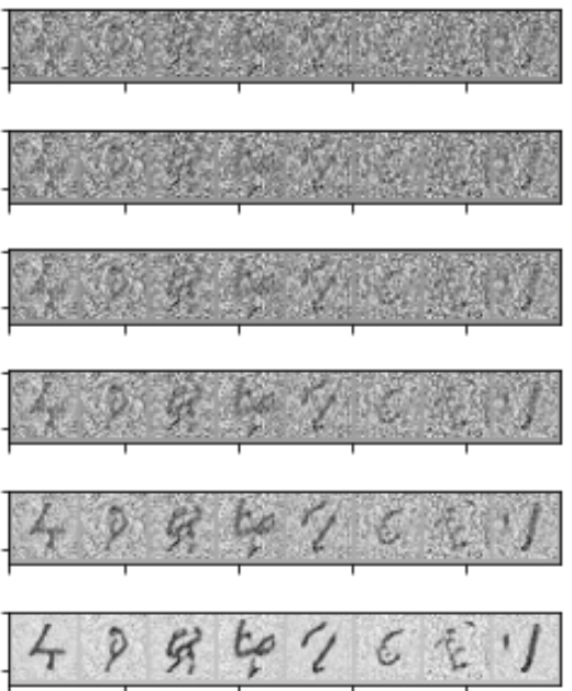
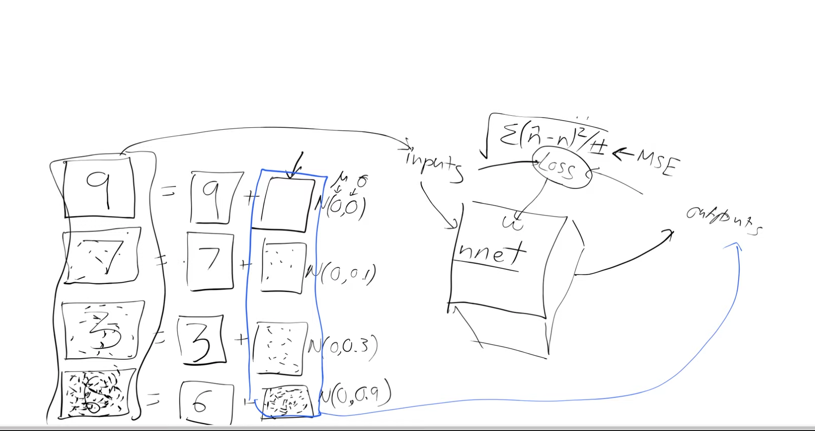
To proceed, we require training data. We generate this data by taking real handwritten digits and overlaying random noise on top of them. Measuring the precise similarity between these noisy images and handwritten digits can be challenging. Instead, we adopt an approach to predict the amount of noise added. For example, the slightly noisy representation of the number seven (depicted in the figure below) can be seen as the original number seven with some additional noise.

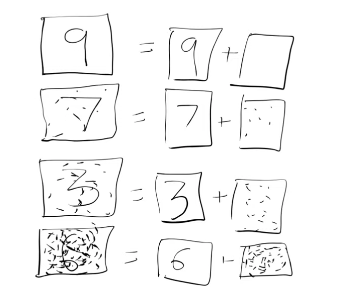
Having generated the data, we don’t assign an arbitrary probability to determine how closely an image resembles a handwritten digit. Instead, we infer that the quantity of noise added inherently indicates the similarity to a digit. For instance, an image with no noise closely resembles a digit (as seen in the example of digit 9 in the figure above), while an image with substantial noise bears little resemblance to a digit (as observed in the example of digit 6 in the figure above).

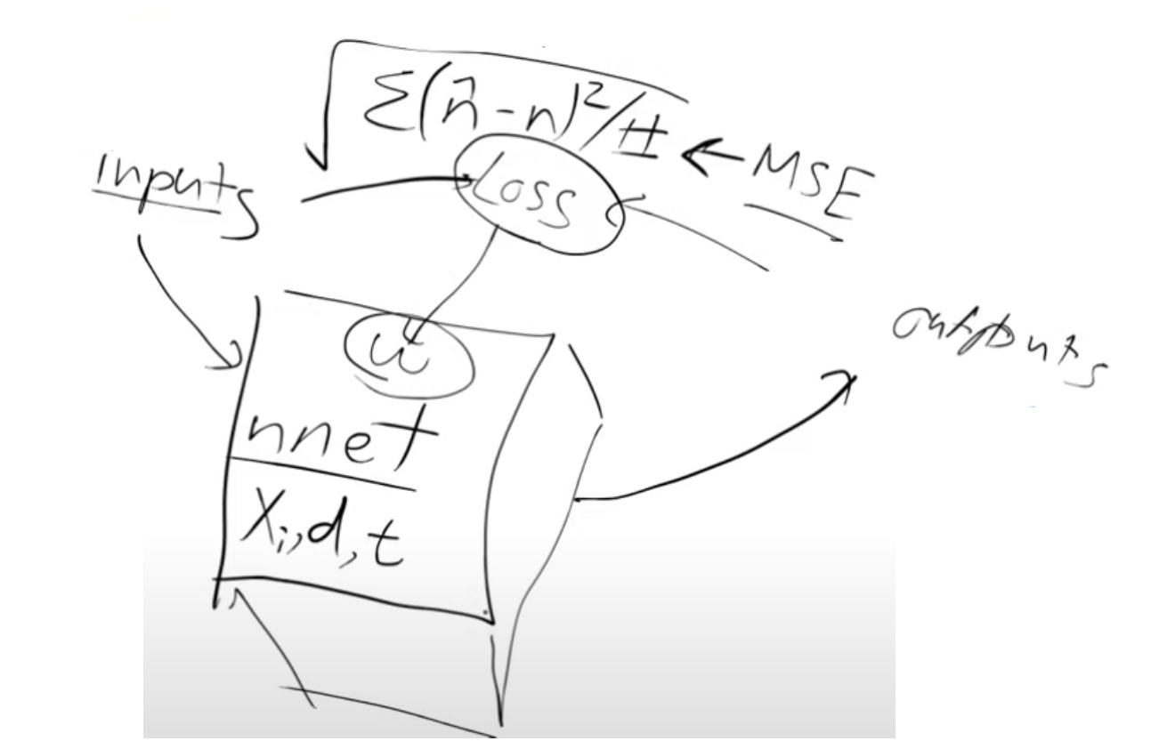
Let’s design a neural network with specific objectives:

• Our neural network takes “noisy digits” as inputs and aims to produce an output representing “noise.”
• To achieve this, we will use the Mean Squared Error (MSE) as our loss function, measuring the difference between the predicted output (noise) and the actual noise.

This setup allows us to determine the precise adjustments needed for each pixel to enhance its resemblance to a digit, which perfectly aligns with our goal \(\nabla(P(X_3)\)

After training the neural network, we can apply it to an image containing random noise. The network will then provide us with valuable information, indicating which parts of the image it perceives as noise while preserving the regions that bear the closest resemblance to digits. However, this process occurs iteratively, rather than in a single step, and the reasons for this will become clear as we delve deeper.

Through training, our neural network acquires the ability to modify noisy input images, refining them to resemble digits more accurately. Consequently, when we pass an image (comprising random noise) through the trained network, it identifies and highlights the areas it considers as noise, leaving behind the parts that best resemble digits. The iterative approach serves specific purposes, which we will explore in more detail later.

Building blocks of stable diffusion

Now that we have established this foundational groundwork, let’s explore the fundamental components that contribute to stable diffusion.

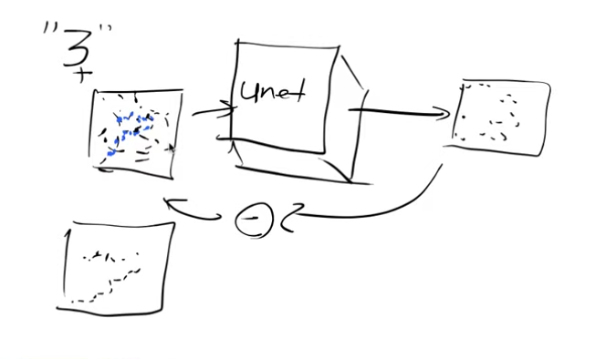
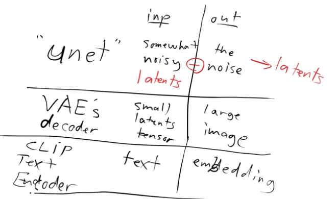
1 - UNET:

Let’s examine the input and output of the Unet model and explore methods to accelerate the training process through compression:

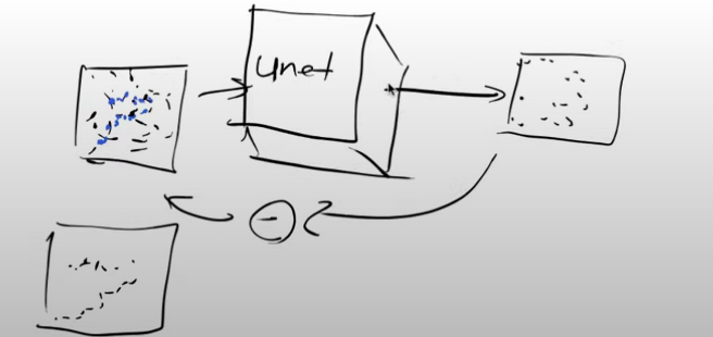
• Input: The input to the Unet is a somewhat noisy image, ranging from minimally noisy to completely noisy.
• Output: The model’s output aims to represent the noise pattern present in the input image.

By subtracting the output noise from the input image, we obtain an approximation of the denoised image.

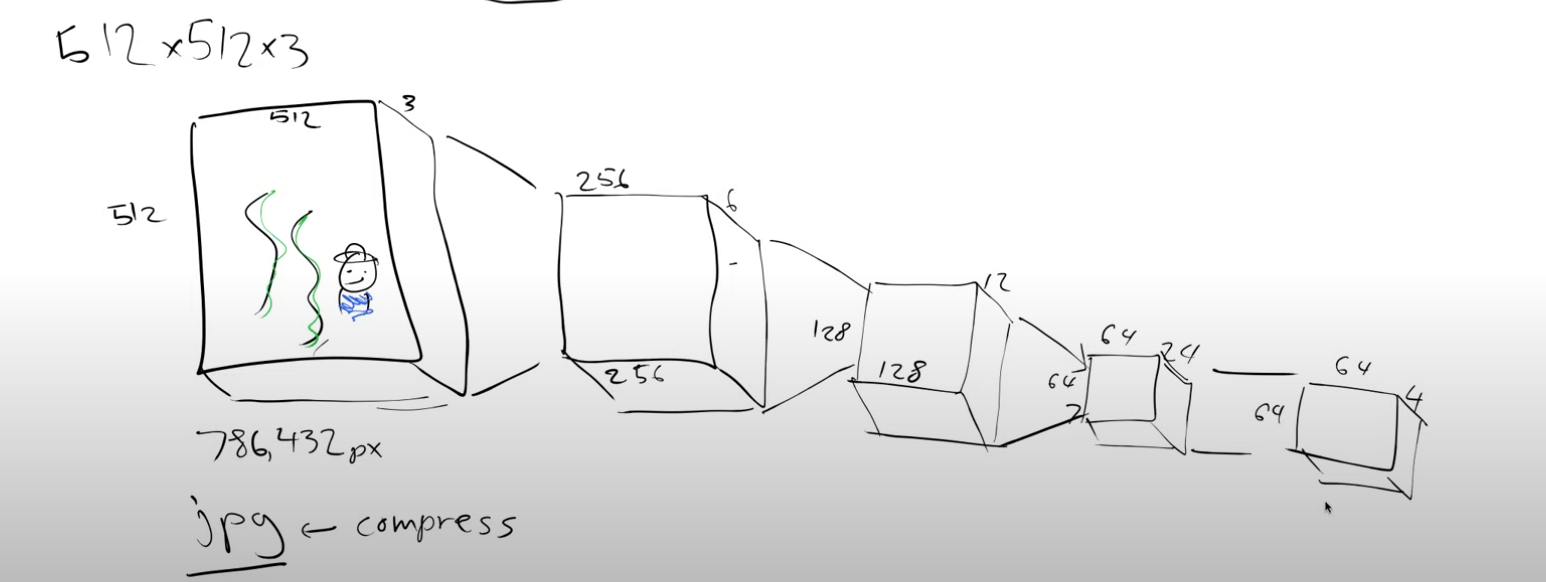
Currently, the handwritten input images are 28x28 in size, but the desired goal is to generate larger images. The Unet models typically work with 512x512x3 images for which millions of noisy versions are used during training. However, training such a model using these large datasets can be time-consuming.

To expedite the training process, we can leverage an insightful approach that capitalizes on the fact that pixel values exhibit minimal local variation. Storing each individual pixel value is unnecessary. Instead, we can utilize compression techniques like JPEG, which significantly reduce the amount of storage required to represent an image while retaining essential information. This compression strategy allows us to achieve faster training without compromising the overall image quality.

2- VAE - Variational autoencoders:

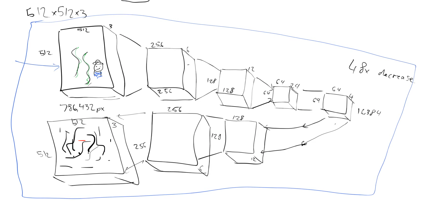
Now, let’s explore the process of compressing it using an autoencoder (AE). The autoencoder’s architecture involves progressively halving the number of pixels per dimension and doubling the number of channels at each level using stride two convolutions. Finally, we incorporate a few ResNet-like blocks to further reduce the channel count from 24 to 4.

We began with a 512x512x3 image and successfully obtained its compressed representation, known as “latents,” which now has a size of 64x64x4. The compression factor achieved is an impressive 48, resulting in a much smaller representation. This encoding process, which transforms the larger image into a compact form, is carried out by the encoder.

The chosen compression factor becomes meaningful based on how effectively we can reconstruct the original image from these 64x64x4 latents. To achieve this, we will develop the inverse process, referred to as the decoder. Once both the encoder and decoder are constructed, they can be combined, and the entire autoencoder can be trained effectively.

In summary, the process involves encoding the “big” image into smaller latents (encoder), followed by decoding those latents back to reconstruct the original image (decoder), and finally, training the complete autoencoder with this setup.

We can use MSE and train this, in the beginning we will get random outputs but later we should get close to our input

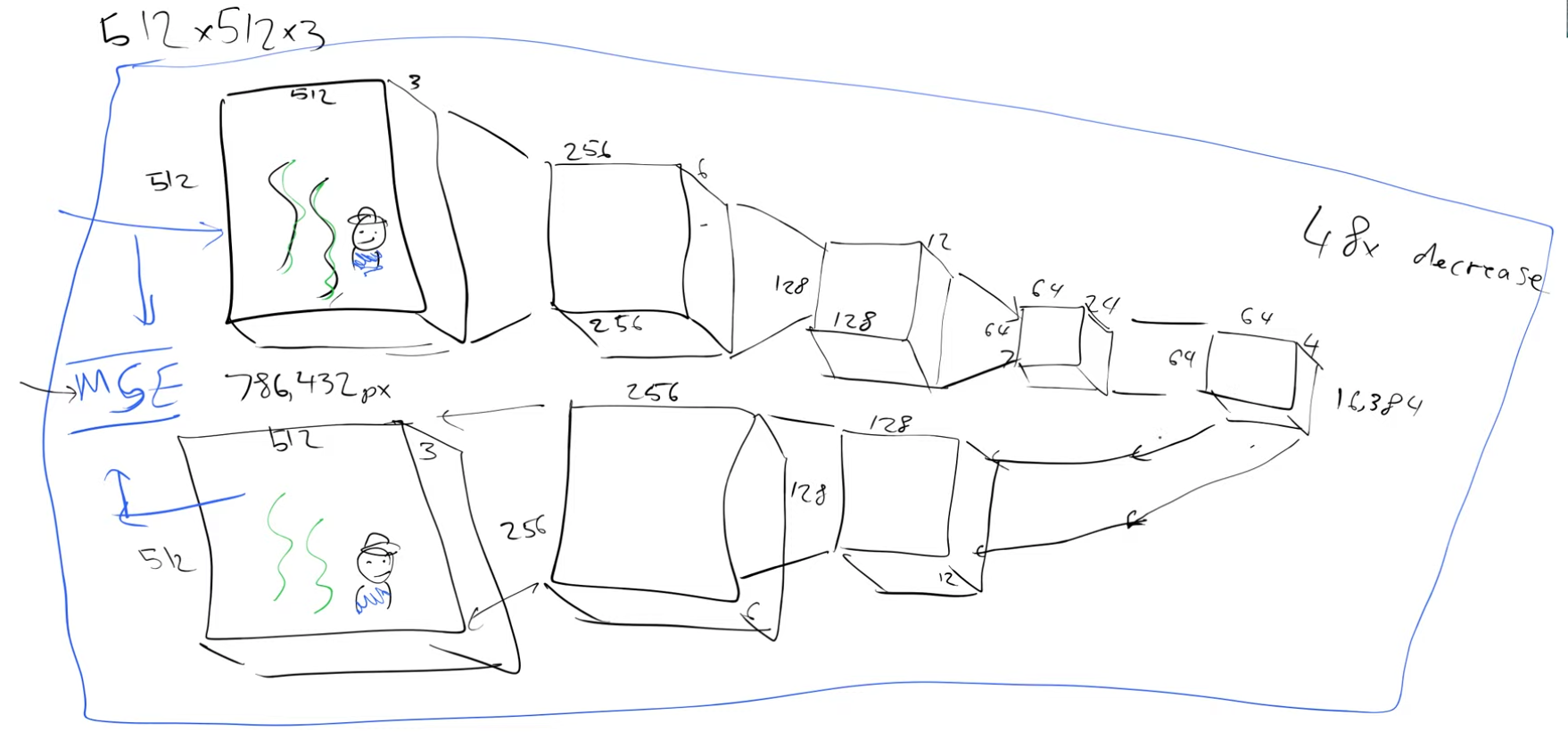
So what is the point of a model that spits back an output that is identical to the input?

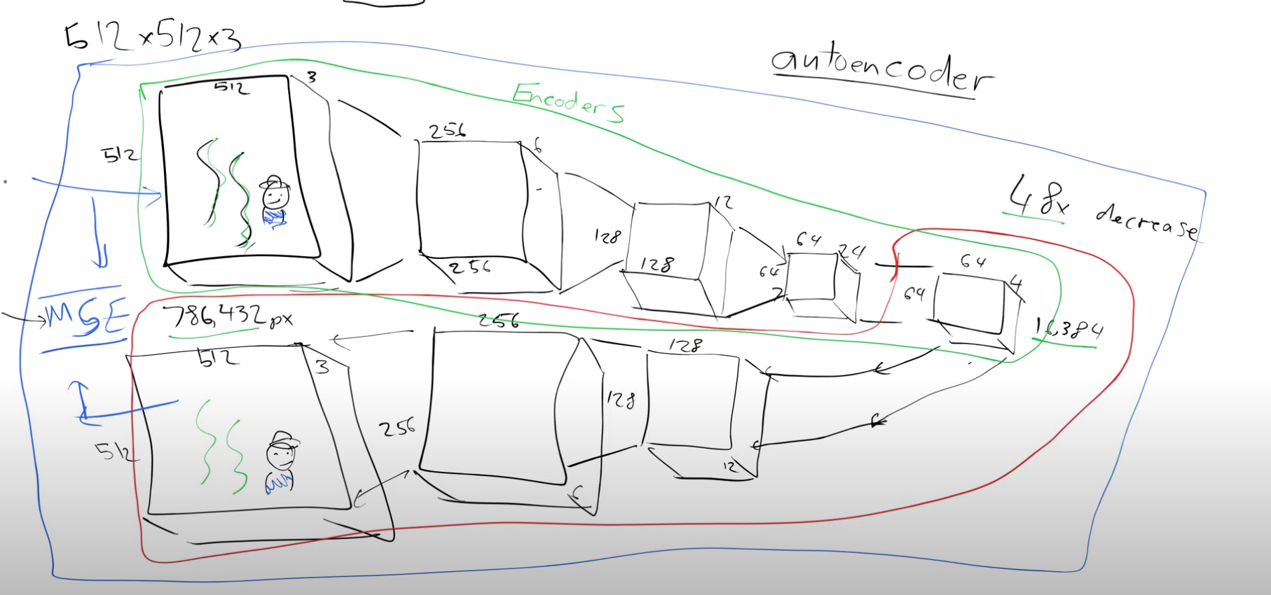
The encoder, depicted in green, is responsible for transforming a larger image into a compact representation. Conversely, the decoder, shown in red, performs the inverse operation, reconstructing the original image from the compressed representation. If I wish to share an image with someone, I can pass it through the encoder, resulting in a representation that is 48 times smaller than the original picture. The recipient, possessing a copy of the trained decoder, can then use it to reverse the process and recover the original image. Essentially, this entire mechanism functions as a compression algorithm, facilitating efficient image transmission and reconstruction.

To utilize the compression algorithm effectively, we employ the Unet by passing the compressed “smaller” latents instead of the original “bigger” images as inputs.

The updated inputs and outputs of the Unet are as follows: - Input: Latents with some level of noise - Output: Noise

By subtracting the output from the input, we obtain denoised latents, which are then fed into the decoder of the autoencoder to generate the best approximation of the denoised image. This autoencoder is called a Variational Autoencoder (VAE).

In summary, the process involves starting with a 512x512x3 image, passing it through the VAE’s encoder to obtain compressed latents of size 64x64x4. Subsequently, these latents are passed through the Unet to predict the noise. The noise is then subtracted from the encoder’s latents, resulting in denoised latents. These denoised latents are finally passed through the decoder of the VAE to generate a 512x512x3 image.

Important points to consider:

• The VAE serves as an optional building block, allowing faster training of the Unet with smaller-sized latents rather than full images.
• During inference, the encoder of the VAE is not required; it is only necessary during the training phase.

3 - CLIP:

Now, let’s explore the significance of text prompts in the process. Instead of merely inputting noise and receiving a digit in return, can we experiment with instructing the system to generate a particular number, for instance, “3”?

To accomplish this, besides providing the noisy input image, we will also include a one-hot encoded representation of the digit “3”.

Currently, we are inputting two elements into this model: the image pixels and the one-hot encoded vector representing the digit it corresponds to. Consequently, the model will learn to predict the noise, benefiting from the extra information about the original digit. This improvement is expected compared to the previous model’s noise prediction capability.

Once the model is trained, feeding it the one-hot encoded vector for “3” along with the noise will enable it to recognize the noise that does not represent the number three. This process is referred to as “guidance,” as it helps the model generate the desired image.

However, one might wonder if one-hot encoded vectors are the most efficient approach. For instance, if we wish to create an image from the phrase “a cute teddy,” using one-hot encoded vectors for every phrase could be highly inefficient.

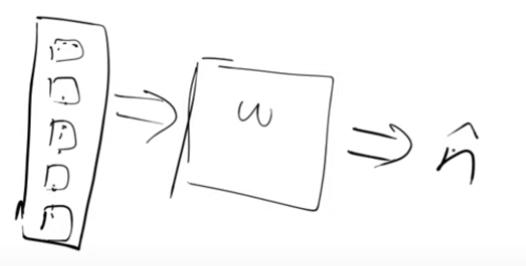
To address this, we can develop a model capable of taking the phrase “a cute teddy” as input and generating a vector of numbers, known as embeddings, which somehow represents the characteristics of “cute teddies.”

In practice, we can obtain images from the internet, where those with alt tags will have associated text descriptions. These descriptions can be leveraged to create meaningful input for the model’s embeddings, enabling it to understand and generate images that align with the given text description.

Now we can create two models, one model which is a text encoder and one model which is an image encoder.

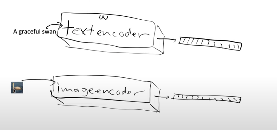
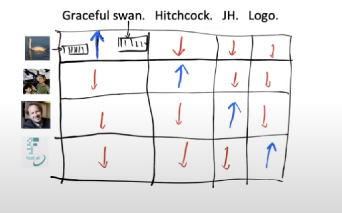
To achieve our goal, we have two encoders—one for processing images and another for handling text. Each encoder produces two embeddings.

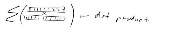
When we pass the image of the swan through the image model, our aim is to obtain embeddings that closely resemble the ones generated by passing the text “the graceful swan” through the text encoder. In essence, we desire similarity between these embeddings. To accomplish this, we leverage the dot product as a measure of similarity. A higher dot product indicates a greater degree of similarity between the embeddings.

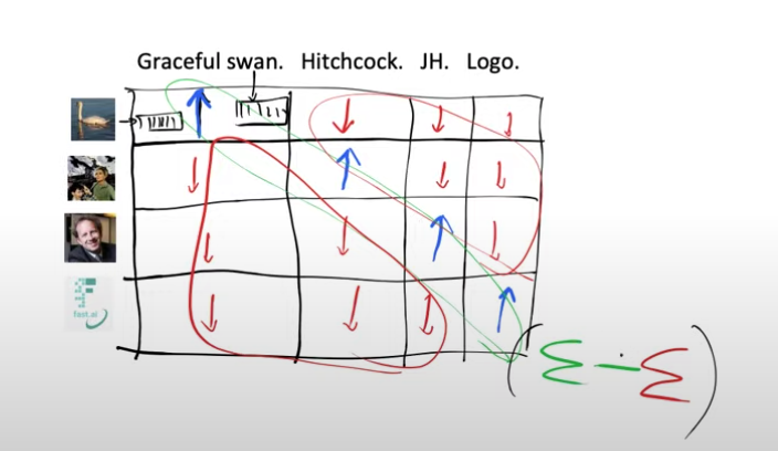
Now, we have a grid containing images and corresponding text, and by computing the dot product of their embeddings, we obtain a score for each combination. Our objective is to achieve high dot product scores (represented by blue diagonal elements) only for matching image-text pairs. Conversely, for non-matching pairs of text and image, we aim to obtain lower dot product scores (depicted by red off-diagonal elements).

So our loss function can be defined as adding all the diagonal elements and subtracting from it the off-diagonal elements.

If we want this loss function to be good then we’re going to need the weights of our model for the text encoder to spit out embeddings that are very similar to the image embeddings that they’re paired with and not similar to the embedding of the images they are not paired with.

Now we can feed our text encoder with “a graceful swan”, “some beautiful swan”, “such a lovely swan” and these should all give very similar embeddings because these would all represent very similar images of swans.

We’ve successfully created two models that put text and images into the same space, a multimodal(using more than one mode-images and text) model.

So we took this detour because creating 1-hot encoded vectors for all the possible phrases was impractical. We can can now take our phrase - “a cute teddy bear” and feed it in text encoder to get out some features/embeddings.

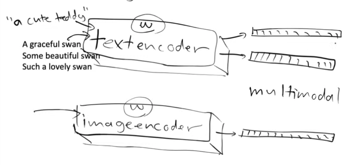
Instead of using 1-hot encoded vectors as guides during Unet training, we utilize the features generated by the text and image encoders. So, when we input the phrase “a cute teddy” into the text encoder, it produces embeddings that serve as guidance for our model to transform the input noisy image into something resembling “cute teddies” it has encountered before.

This pair of models is known as CLIP, which stands for Contrastive Language-Image Pre-training, and the loss function employed is called contrastive loss.

Let’s now review the building blocks we have established so far.

• we’ve got a Unet that can denoise latents into unnoisy latents
• we’ve got the decoder of VAE that can take latents and create an image
• we’ve got the CLIP text encoder which can guide the Unet with captions

Stable diffusion is a latent diffusion model and what that means is that it doesn’t operate in the pixel space, it operates on in the latent space of some other autoencoder model and in this case that is a variational autoencoder.

4 - Additional Things:

There are two more things Jeremy talks about: - Score function - time-steps

These gradients are commonly referred to as the “score function.”

The term “time steps” is frequently found in various papers, although we did not employ any actual time steps during our training process. This terminology originated from the initial mathematical formulations. Despite this, we can understand the concept of time steps without it being directly related to real-world time.

During training, we introduced diverse levels of noise to our images, varying from highly noisy to noise-free and even pure noise.

To establish a noising schedule, we utilize a monotonically decreasing function. Let’s consider the x-axis (“t”) ranging from one to a thousand. We randomly select a number within this range and use the noise schedule to determine the corresponding sigma (also referred to as beta in some papers). For instance, if we randomly choose the number four, we would look up the corresponding sigma value on the y-axis, representing the amount of noise to add to the image with this randomly chosen value of four.

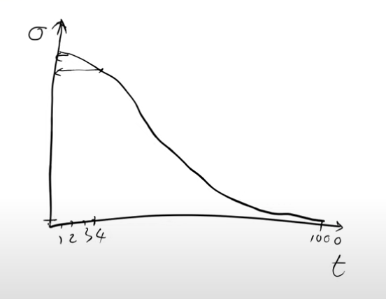
During the training process, the level of noise added to each image varies depending on a random selection. If a value close to one is chosen, the resulting image will have a substantial amount of noise, whereas a value near one thousand will lead to minimal noise.

To achieve this randomness in training, we need to determine a random amount of noise for every image. This can be achieved by selecting a random number between one and a thousand and using a noise scheduler function to obtain the corresponding sigma value for the noise to be added.

Previously, people often referred to this random number as the “time step,” but nowadays, the noise scheduler lookup is becoming less prevalent. Many practitioners now simply state the magnitude of noise used.

During the training process, for each mini-batch, a random batch of images is selected from the training set. Additionally, either a random amount of noise or a random “t” value (which is then used to find the amount of noise from the noise scheduler) is chosen. These noisy images are then passed into the model for training, allowing the model’s weights to learn how to predict noise effectively.

How do we precisely carry out this inference process? When generating a picture from pure noise, it corresponds to t=0 on the noise scheduler, representing maximum noise. The objective is to teach the model to eliminate noise effectively. However, attempting to accomplish this in a single step could result in poor-quality images.

In practice, the noise prediction is multiplied by a constant “c,” akin to a learning rate, but here it is not updating model weights; rather, it updates individual pixels. This updated prediction is then subtracted from the original noisy pixels, resulting in a slightly denoised image.

However, the model does not immediately reach the final denoised image because certain image characteristics, such as those appearing with t=1 (which correspond to poor-quality images), were not encountered in the training set. Consequently, the model lacks knowledge on how to handle such images. To address this, only a small factor of the noise is subtracted, ensuring that the process repeats with somewhat noisy latents, allowing the model to iterate and refine the denoising gradually.

Deciding the appropriate value for “c” and determining how to perform the subtraction from the noise prediction are vital aspects addressed in the actual diffusion sampler. The sampler manages both the addition of noise and the subsequent subtraction during the diffusion process.

Interestingly, this approach bears resemblance to deep learning optimizers. For instance, momentum in optimizers suggests increasing the change in parameters when they are changed repeatedly by a similar amount over multiple steps. Similarly, Adam optimizer considers changes in variance. Although diffusion-based models and optimizers stem from different mathematical domains (differential equations versus optimization), they share parallel concepts. Differential equation solvers also focus on taking more significant steps to converge quickly. They often utilize t as an input, a common feature in most diffusion models, although we have yet to discuss it in detail.

In diffusion models, it’s a common practice to include not only the input pixels and captions but also the parameter “t.” The intention behind incorporating “t” is to provide the model with information about the amount of noise present, as “t” is associated with the noise level.

However, Jeremy strongly suspects that this premise might be incorrect because for a sophisticated neural network, determining the noise level can be relatively straightforward. Consequently, when the need for passing “t” diminishes, the problem transforms from one resembling differential equations to that resembling optimizers.

By swapping Mean Squared Error (MSE) with perceptual loss, various possibilities emerge, expanding the approach to be viewed as an optimization problem rather than merely a differential equation-solving problem. This shift in perspective unlocks new avenues for exploration and potential improvements in the model’s performance.